Robust portfolio optimization under uncertainty

Build an allocator, hand it three datasets it has not seen, and be scored on how it does. The universes ranged from 15 to 40 assets across finance, technology and healthcare, described by eight factor returns, rebalanced over twenty periods.

Two things were scored: the Sharpe ratio, at eighty percent of the weight, and the turnover ratio, at the remaining twenty. Runtime had to stay under five minutes. Because the evaluation ran on held-out trials, anything tuned to the training window was a liability rather than an advantage.

We compared three families of allocator and then tried to improve the best one. My part was the robust ellipsoidal Sharpe formulation, the sparse LASSO factor estimator, and the Sharpe-CVaR hybrid, all in CVXPY.

Estimating the inputs

Mean-variance style optimisers are acutely sensitive to their inputs. Small errors in the estimated mean or covariance move the weights a long way, which is how an allocator ends up rebalancing violently every period and paying for it in turnover.

Sample means and covariances are the unstable option. A multifactor model is the more stable one, describing each asset’s return through a small number of shared factors, but including too many factors reintroduces the overfitting it was meant to solve. Penalising the factor loadings with an L1 norm keeps the model sparse and selects the factors that carry the asset.

\min_{B_i} \; \bigl\| r_i - X B_i \bigr\|_2^{2} \;+\; \lambda \bigl\| B_i \bigr\|_1

Estimates of expected return and covariance are then rebuilt from the sparse loadings rather than from the sample statistics.

Robustifying the objective

Maximising the Sharpe ratio directly is not convex. Reparameterising it removes that problem, and an ellipsoidal uncertainty set around the estimated returns handles the fact that those estimates are wrong by some amount. The parameter ε sets how much error the allocator assumes it is working with.

\min_{y} \; y^{\mathsf T} Q y \quad \text{s.t.} \quad (\mu - \bar r_f)^{\mathsf T} y - \epsilon_2 \bigl\| \Theta^{1/2} y \bigr\|_2 \;\ge\; 1, \quad \mathbf{1}^{\mathsf T} y \ge 0, \quad y \ge 0

Portfolio weights are recovered afterwards by normalising y.

The three baselines

Each model was run unmodified first, to get a reference for both scored quantities. Values are given per dataset.

Model	Sharpe	Turnover
Sharpe ratio	0.165 / 0.138 / 0.235	0.585 / 0.667 / 0.682
Risk parity	0.189 / 0.200 / 0.212	0.170 / 0.130 / 0.205
CVaR	0.212 / 0.088 / 0.222	0.812 / 0.845 / 0.835

Risk parity produced the steadiest weights, which is what it is designed to do, and the lowest turnover of the three. CVaR reached a competitive Sharpe on two datasets but rebalanced hardest, and collapsed on the second dataset. Sharpe optimisation sat in between.

What actually improved the score

Applying the sparse LASSO estimator to the robust Sharpe model changed one quantity far more than the other.

	Sharpe	Turnover
Sharpe, baseline	0.165 / 0.138 / 0.235	0.585 / 0.667 / 0.682
Robust Sharpe + LASSO	0.202 / 0.182 / 0.201	0.087 / 0.048 / 0.084

Sharpe improved modestly and fell slightly on the third dataset. Turnover fell by roughly a factor of seven. Since a sparse factor model produces expected returns that move less between periods, the optimiser has less reason to reshuffle the portfolio, and the trading cost implied by the turnover ratio drops with it.

That comparison changes two things at once, the objective and the estimator, so it is worth separating them. Re-running the second dataset with the robust Sharpe objective held fixed and only the estimator swapped gives 0.228 turnover from sample estimates against 0.048 from sparse ones, at Sharpe 0.164 and 0.182. Most of the effect is the estimator. The weights show it directly.

Stacked portfolio weights over twenty rebalance periods using sample factor estimates, showing large shifts between periods — **Figure 1.** Portfolio weights across the twenty rebalance periods of the second dataset, same optimiser both times. Each band is one of the thirty assets, so a band that changes width is a position being bought or sold. Sample estimates on the left keep rewriting the portfolio; sparse estimates on the right mostly leave it alone.

Stacked portfolio weights over twenty rebalance periods using sparse LASSO factor estimates, showing nearly flat bands — **Figure 1.** Portfolio weights across the twenty rebalance periods of the second dataset, same optimiser both times. Each band is one of the thirty assets, so a band that changes width is a position being bought or sold. Sample estimates on the left keep rewriting the portfolio; sparse estimates on the right mostly leave it alone.

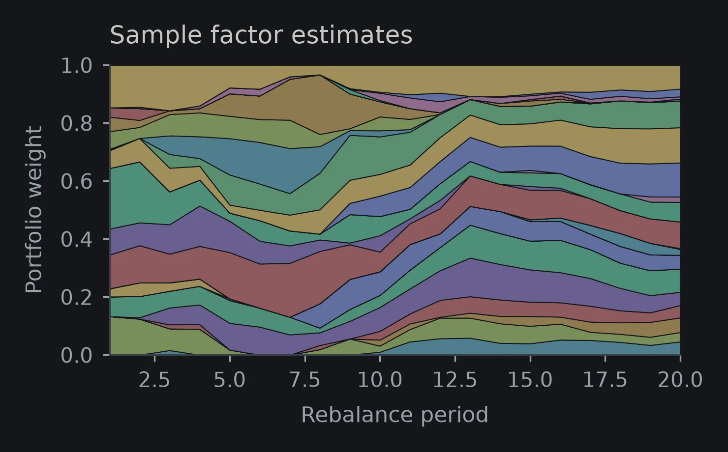
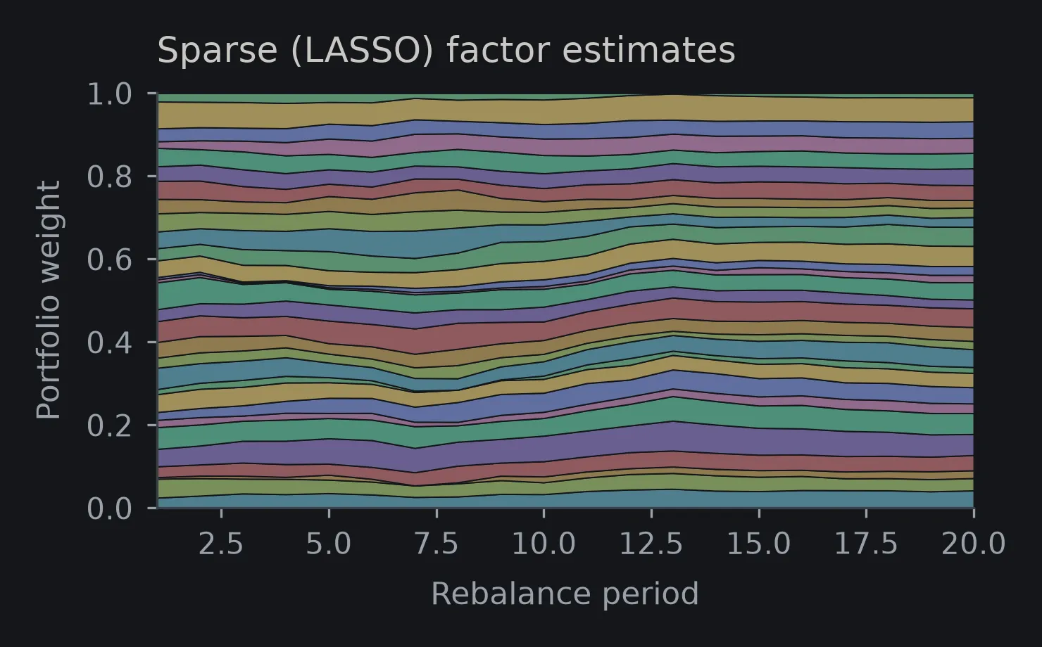
Two further variants did not survive. Risk parity and a relaxed CVaR moved the Sharpe ratio a little in both directions but degraded turnover enough to lose on aggregate. Layering CVaR on top of the robust LASSO model degraded turnover by about an order of magnitude, which no Sharpe improvement was going to cover.

The selected model ran in 0.29 seconds against a five-minute limit.

Result

Across two held-out trials the allocator placed 5th and 2nd of 10 groups. The spread between those two placings is worth stating plainly: the datasets were different, and a model that ranks mid-table on one and near the top on another has not demonstrated that it is reliably better than the alternatives.

What I would do differently

The penalty weight λ and the uncertainty parameter ε were chosen by validation over a small grid. Both control how much the model distrusts its own inputs, and they interact, so a joint sweep would have been better than tuning them in sequence.

We also evaluated on three datasets from one era. Turnover reduction from sparsity should hold generally, but the Sharpe figures are specific to these samples and I would not extrapolate them.

MIE377_Fin_Opt_Algo_Trading on GitHub →

Three-person team with Eric Toma and Carter Buck. We co-authored the report; the robust Sharpe formulation, the LASSO estimator and the Sharpe-CVaR hybrid were mine.

← All work