Reward design in a multi-agent market

Ten agents start a trading day holding a position they did not choose. Five are long fifty thousand shares, five are short fifty thousand. They have 120 ticks to get flat, and their only counterparties are each other.

The task is narrow enough that a good outcome is unambiguous, which makes it a clean setting for the question I was interested in: how much the wording of the reward function changes what the agent does. I designed four reward and cost specifications and ran them against each other on the same environment.

The four specifications

Notation: q is inventory, p the mid price, t the tick, T the tick limit of 120, and N the agent’s initial capital at risk. ΔPnL is the change in total profit and loss over the tick, inclusive of costs.

PnL Only

Profit, normalised by capital at risk, and nothing else.

r_t \;=\; w\,\frac{\Delta \mathrm{PnL}_t}{N}, \qquad w = 2

PnL Focused

Adds a term for reducing the position, and a fee on inventory held near the end of the day that steps up twice.

r_t \;=\; w\,\frac{\Delta \mathrm{PnL}_t}{N} \;+\; \lambda\,\bigl(|q_{t-1}| - |q_t|\bigr)\frac{p_t}{N} \;-\; \varphi(t)\,\frac{|q_t|}{N}

w = 1, λ = 0.05. The fee φ(t) is 0.01 over the last 30 ticks and 0.02 over the last 10, and zero before that.

Quadratic Inventory

The same shape, with the late fee quadratic in inventory and ramping quadratically in elapsed time.

r_t \;=\; w\,\frac{\Delta \mathrm{PnL}_t}{N} \;+\; \lambda\,\bigl(|q_{t-1}| - |q_t|\bigr)\frac{p_t}{N} \;-\; \varphi(t)\,\frac{q_t^{2}}{N}, \qquad \varphi(t) = \kappa\left(\frac{t - t_{\mathrm{late}}}{T - t_{\mathrm{late}}}\right)^{2}

w = 1, λ = 0.1, κ = 5e-4, with the penalty starting at t_late = T − 30.

Quadratic Cost

The reward function here is PnL Only, unchanged and at the same weight. The quadratic inventory term moves out of the reward and into the cost function, where it is charged every tick and enters ΔPnL.

c_t \;=\; c\,q_t^{2}, \qquad c = 10^{-4} \qquad\qquad r_t \;=\; w\,\frac{\Delta \mathrm{PnL}_t}{N}, \qquad w = 2

Charged from the first tick, with no time gate and no normalisation.

Quadratic Cost and PnL Only differ in that substitution and in nothing else.

Effect on the position

Long trader mean inventory under four reward specifications — **Figure 1.** Mean inventory for the two sides of the book, seeded equal and opposite. The ordering follows the strength of the inventory penalty: both quadratic specifications are flat by step 55, the P&L-focused one by step 120, and the profit-only agent settles around fifteen hundred shares and stays there. Smoothed with a time-weighted EMA at 0.97; the raw series is faded behind each line.

Short trader mean inventory under four reward specifications — **Figure 1.** Mean inventory for the two sides of the book, seeded equal and opposite. The ordering follows the strength of the inventory penalty: both quadratic specifications are flat by step 55, the P&L-focused one by step 120, and the profit-only agent settles around fifteen hundred shares and stays there. Smoothed with a time-weighted EMA at 0.97; the raw series is faded behind each line.

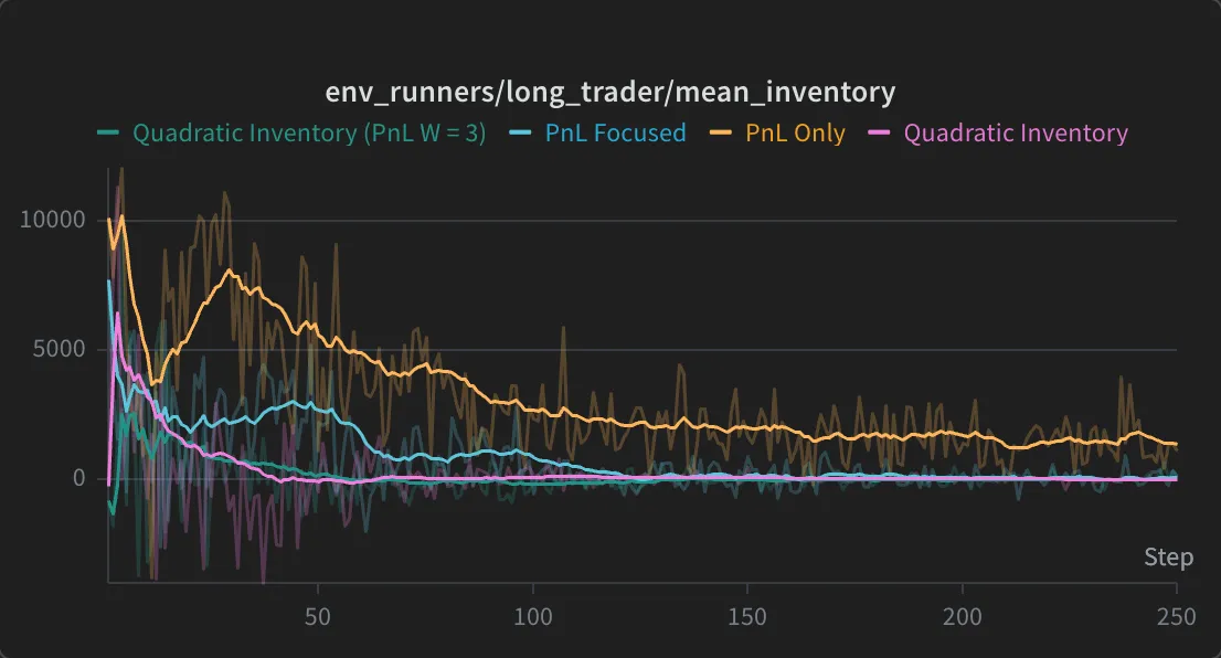
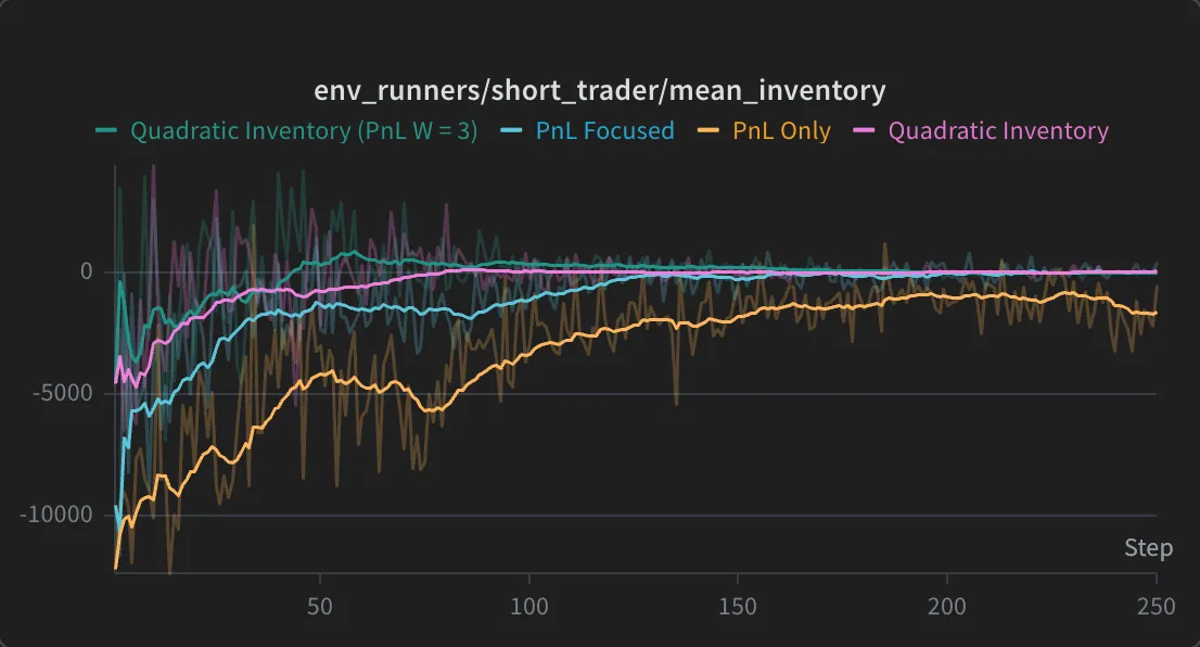
Two qualifications. This is inventory averaged over the episode rather than the position at the close. Every specification ends flat, at a final inventory of zero, so the chart measures how quickly each unwinds and not whether it does.

The two agents are plotted separately because they are seeded equal and opposite. A persistent long on one side and a persistent short on the other cancel in the aggregate, which makes the aggregate series uninformative here.

Effect on profit and loss

Mean total P&L under five reward specifications — **Figure 2.** Mean P&L across all five runs on the left. Quadratic Cost reaches −12,500,000, about three hundred times the range of the other four, which compresses them to a line at zero. The right panel is the same metric with that run hidden: the axis rescales to −40,000, and the P&L-focused specification is the only one that finishes positive.

Mean total P&L under four specifications, quadratic cost hidden — **Figure 2.** Mean P&L across all five runs on the left. Quadratic Cost reaches −12,500,000, about three hundred times the range of the other four, which compresses them to a line at zero. The right panel is the same metric with that run hidden: the axis rescales to −40,000, and the P&L-focused specification is the only one that finishes positive.

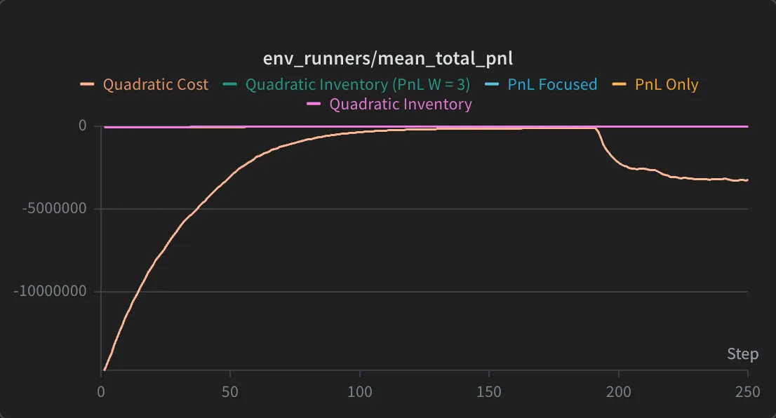
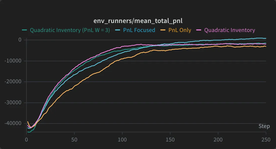
Why the substitution matters

Moving the quadratic term from the reward to the cost function changes two things, and both increase its magnitude.

It loses its normalisation. On the reward side the penalty is divided by N, the agent’s initial capital at risk. On the cost side it is charged in raw currency, so an identical coefficient of 10⁻⁴ represents a much larger quantity.

It also loses its time gate. The reward-side penalty is inactive until the last 30 ticks and ramps in quadratically. The cost-side penalty applies from the first tick at full strength.

At the twenty-thousand-share position the agent reaches, the per-tick charge is 10⁻⁴ × 20,000² = 40,000, sustained over 120 ticks, which accounts for the observed magnitude.

Generally: a penalty that is well behaved as a normalised reward term is not well behaved as an unnormalised cost at the same coefficient, and in a configuration file the two are hard to tell apart.

A result that came from a bug

Earlier single-agent runs produced a total P&L averaging +12,639, with the profit coming almost entirely from an opening block trade, after which the agent unwound and held the gain.

The position limit was enforced against current inventory rather than post-trade inventory:

if inventory > max_inventory and action_type == 1:
    return True

An agent sitting exactly at the limit could therefore buy again and exceed it, and the policy built its strategy around that. The corrected check tests the position the order would produce:

if action_type == 1 and inventory + shares > max_inventory:
    return True

The same commit corrects a second instance of the error. The blocked-buy and blocked-sell flags in the agent’s observation vector were off by one in the same direction, so the agent was also being told it was free to trade while at the limit. The team write-up documents the enforcement side; the observation side is not mentioned in it.

	Total P&L	Final inventory
Before the fix	+12,639 (sd 6,688)	0.00
After the fix	−2,047 (sd 2,848)	0.00
After retuning	−92 (sd 2,574)	0.00

Produced by the analyzer over run outputs that no longer exist, and not reproduced since.

Correcting the environment moved the result from positive to negative, and the negative figure is the one I would report.

Limitations

Episode-return metrics are measured in reward units, and these runs use four different reward functions, so a higher episode return can reflect scaling rather than performance. Every comparison above rests on total P&L and inventory, which are in currency and shares.

There is one seed per configuration and no sweep. The Quadratic Cost mechanism is arithmetic and I am confident in it; the ordering among the other three is a single observation.

Training budgets differ between runs. Comparisons are made at matched step counts, and the two figures above span the same range.

Attribution

mktsim is Professor Ing-Haw Cheng’s platform. He wrote the simulator, the environment, the reward and cost registry, the normalisation helper, and a set of sample reward and cost functions, accounting for 303 of 332 commits across all branches.

My contribution is the four specifications compared here and the environment fixes described above. The platform’s sample rewards are static functions of state with no notion of elapsed time; the time-dependent penalties in the project, including the stepped late-episode fee, the quadratic ramp, and the liquidation-progress term, were added by me or by Faraaz Ahmed. Faraaz built the analyzer, the experiment logging, and the correlation and action analysis tooling. The project was a four-person team supervised by Prof. Cheng.

I did not build the simulator, the order book, or the team’s architecture.

← All work